How to Insert an Excel 2013 Table
Our article continues below with additional information on how to make a table in excel 2013 and pictures of these steps, as well as information on formatting and filtering your table. Adding data to a spreadsheet in Excel 2013 gives you the ability to sort data, edit it, and perform a number of different mathematical operations and functions on it. But occasionally you might have data that needs some additional formatting or filtering options, in which case it’s helpful to know how to make a table in Excel 2013. Our tutorial below will show you how to create a table from data in your spreadsheet, then customize the design of that data, filter it, or even convert it back into a standard range if you decide that you don’t need or don’t like the table layout. So continue below and find out how to make a table in Excel 2013. Our Microsoft Excel add column tutorial can show you a simple way to get a total for the data in a column if you aren’t using a table.
How to Create a Table in Excel 2013 (Guide with Pictures)
The steps in this article are going to show you how to select data in a Microsoft Excel spreadsheet and convert it into a table. Once you have created a table in Excel 2013 you will be able to customize the design of that table, or filter it so that only some of the data appears in the table. For the sake of this guide we will assume that you already have the data in your spreadsheet, and that the data has headers. If you don’t have headers (a row at the top of the spreadsheet that identifies the data in the columns) then you may want to add a header row to make this process a little easier.
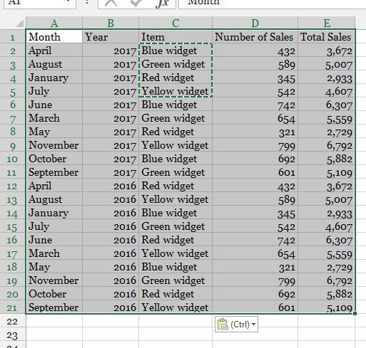
Step 1: Open the spreadsheet in Excel 2013 that contains the data you want to turn into a table.
Step 2: Select the data in the spreadsheet that you wish to turn into a table.
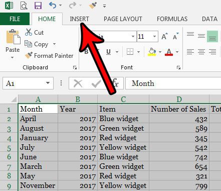
Step 3: Click the Insert tab at the top of the window.
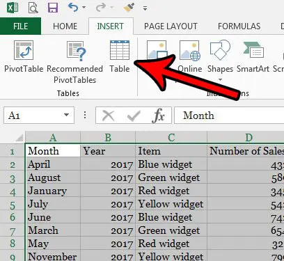
Step 4: Select the Table option.
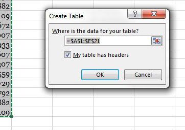
Step 5: Check the box to the left of My table has headers (if it’s not already checked) then click the OK button.
Now that you have turned some of your data into a table and you know how to make a table in Excel 2013, it’s likely that you will want to change the way that it looks. This can include things like changing row or column columns, or automatically alternating row colors.
How to Change the Appearance of Your Table in Excel 2013
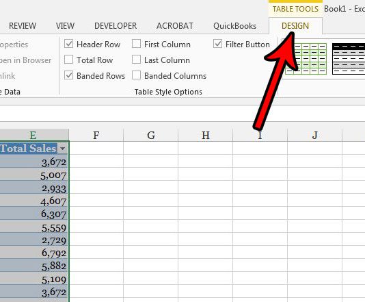
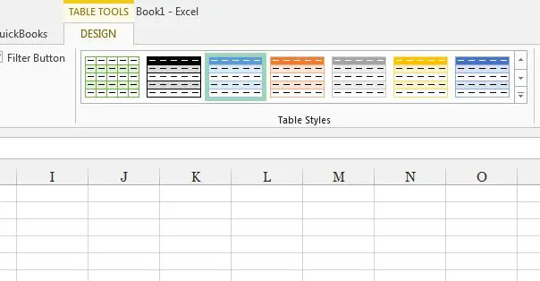
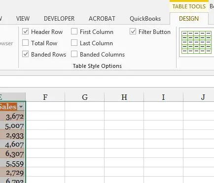
Now that you have created a table in your spreadsheet, it’s a good idea to customize its appearance. This section will show you how to adjust the design of the table to make it look better and make it easier to work with. Step 1: Select the entire table, then click the Design tab at the top of the window. Step 2: Select one of the designs from the Table Styles section of the ribbon. Step 3: Check or uncheck any of the options in the Table Style Options section of the ribbon. For reference, these options mean:
Header Row – check this box if your table has a header row, which identifies the information contained in each columnTotal Row – Check this box to include a Total cell at the bottom of the table for the rightmost columnBanded Rows – Check this option if you want the colors of the table rows to alternate automaticallyFirst Column – Check this option to bold all of the values in the first columnLast Column – Check this option to bold all of the values in the rightmost columnBanded Columns – Check this option to alternate the colors of each row. This can conflict with the Banded Rows option, so it’s typically best to choose one or the other.Filter Button – Check this box to add a dropdown arrow to the right of each column heading which lets you perform the filtering options we will discuss in the next section.
Tables in Microsoft Excel do more than just look good. You also gain access to a variety of powerful filtering tools that can make it much easier to sort and display specific data.
How to Filter a Table in Excel 2013
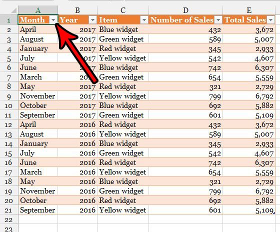
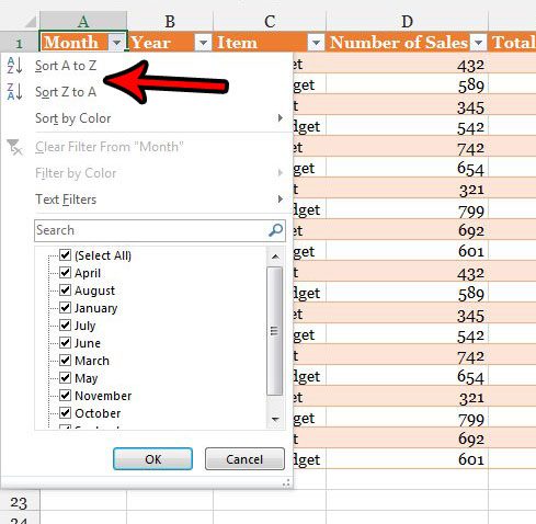
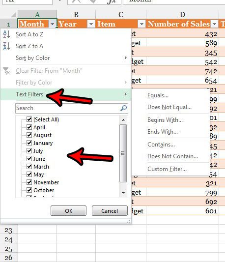
The steps in this section are going to show you how to use the filtering capabilities of the table that you have created. if you don’t see the filtering dropdown menu that we will be using, make sure that you are using header rows, and that you have checked the Filter Button option discussed in the previous section. Step 1: Click the dropdown arrow to the right of the column header for the column data that you want to filter. Step 2: Choose the Sort A to Z option to filter the data in that column with the smallest value at the top, or choose the Sort Z to A option to filter the data with the largest value at the top. Alternatively you can select the Sort by Color option if you have set custom colors for different rows and want to sort that way. Step 3: Select the Text filters option and choose one of the items there if you wish to filter your data in this manner, or check and uncheck values in the list at the bottom to display or hide certain values. If you’ve created and modified the table, you may discover that it isn’t actually what you were looking for. The section below will show you how to change it back to a standard group of Excel cells.
How to Delete the Table and Convert it Back to a Range
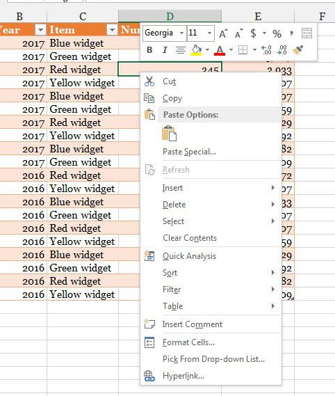
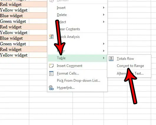
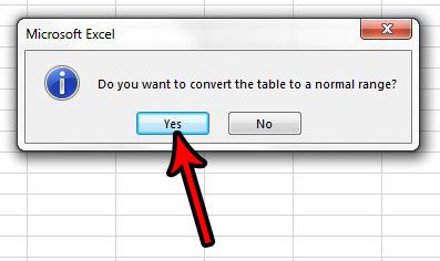
The steps in this section will show you how to remove the table formatting and turn it back into a standard range like it was before you turned it into a table. This won’t delete any of the data in the table, but will remove the filtering options and any design or these settings you have created. Step 1: Right-click one of the cells in the table to bring up the shortcut menu. Step 2: Select the Table option, then choose the Convert to Range option. Step 13: Click the Yes button to confirm that you would like to convert the table back to a normal range. If you have reverted back to a standard range because the table wasn’t what you wanted, then you may want to consider trying a Pivot Table instead. If you select your data again, then click the Insert tab and choose Pivot Table you will be provided with some additional ways to work with your data that may be more beneficial. One of the biggest frustrations that comes from working with Excel is when you need to print. Check out our Excel printing guide that will give you some tips on ways to improve the printing process for your spreadsheets.
See also
How to subtract in ExcelHow to sort by date in ExcelHow to center a worksheet in ExcelHow to select non-adjacent cells in ExcelHow to unhide a hidden workbook in ExcelHow to make Excel vertical text
After receiving his Bachelor’s and Master’s degrees in Computer Science he spent several years working in IT management for small businesses. However, he now works full time writing content online and creating websites. His main writing topics include iPhones, Microsoft Office, Google Apps, Android, and Photoshop, but he has also written about many other tech topics as well. Read his full bio here.
You may opt out at any time. Read our Privacy Policy